Using Poisson and Negative Binomial models to determine what factors link most significantly to the number of exoplanets in a star system.

Background

Formation of stars, exoplanets, and the systems they inhabit have long been the topic of scientific research. Studying what kinds of factors contribute most heavily to the number of exoplanets in a star system can help us to understand why some systems have more planets than others. This project was done as a class project for a course on statistical modeling - as such, I employed both Poisson and Negative Binomnial models to the data.

The Data

The dataset used for this project comes from the NASA Exoplanet Archive.

Variable	Description	Explanation
sy_pnum	Number of planets in the system	Response variable
sy_snum	Number of stars in the system	How many stars are in the system (there can be more than one!)
st_mass	Stellar mass	The weight of the star compared to the Sun
st_rad	Stellar radius	The size of the star compared to the Sun
st_lum	Stellar luminosity	How bright the star is compared to the Sun
st_met	Stellar metallicity	How much heavy elements (like iron) the star has
pl_orbper	Orbital period	How long a planet takes to orbit its star (in days)
pl_orbsmax	Semi-major axis	The average distance between the planet and the star (in AU)
pl_orbeccen	Eccentricity	How oval-shaped the planet’s orbit is (0 = circle, 1 = line)
st_age	Stellar age (in gigayears)	How old the star is, in billions of years
pl_insol	Insolation flux	How much sunlight a planet gets compared to Earth
st_logg	Stellar surface gravity	The strength of gravity on the star’s surface
st_dens	Stellar density	How tightly packed the star’s material is

Exploratory Data Analysis (EDA)

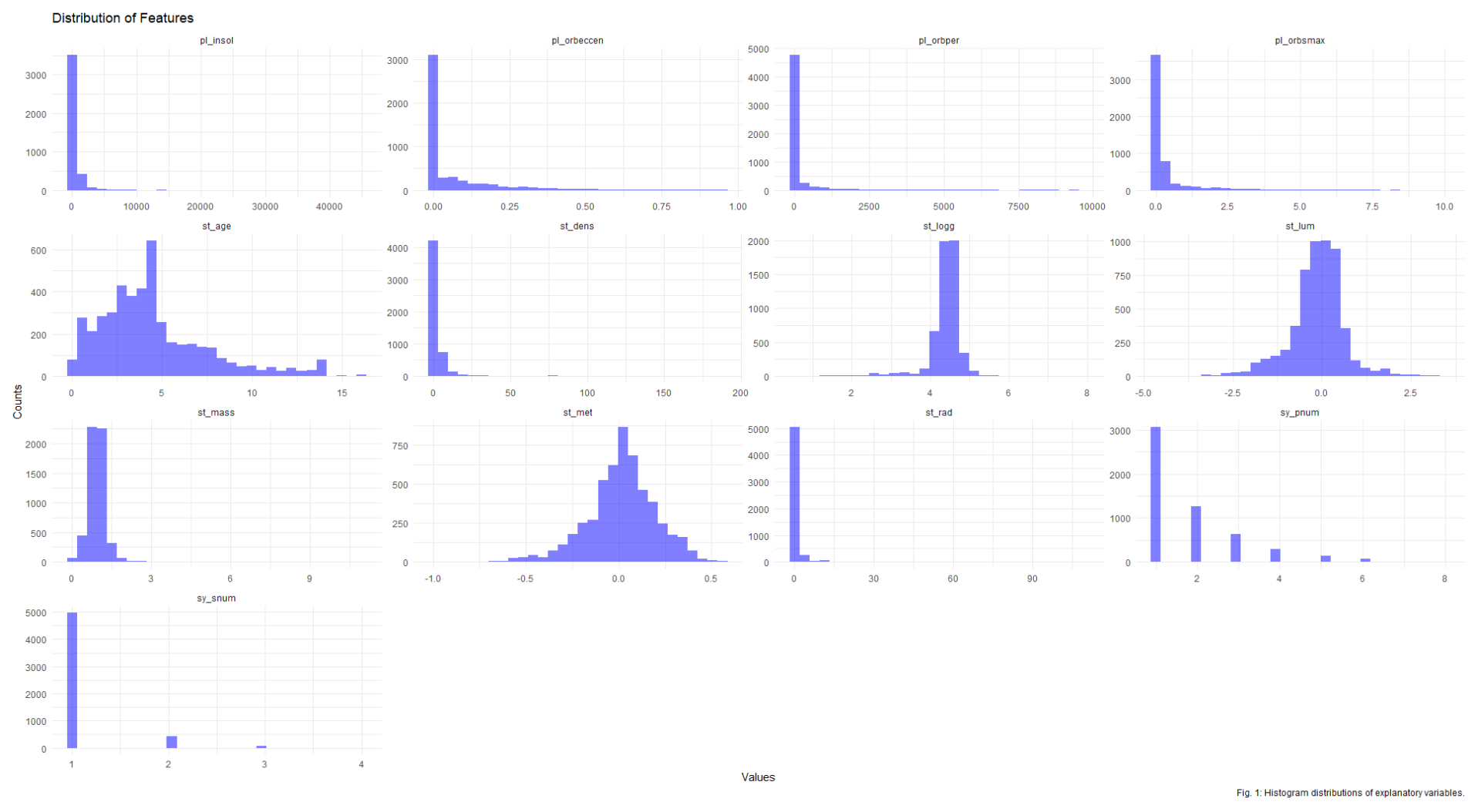
The first EDA plot I made was a simple group of histograms - it’s nice to be able to visually look at summary statistics across several variables.

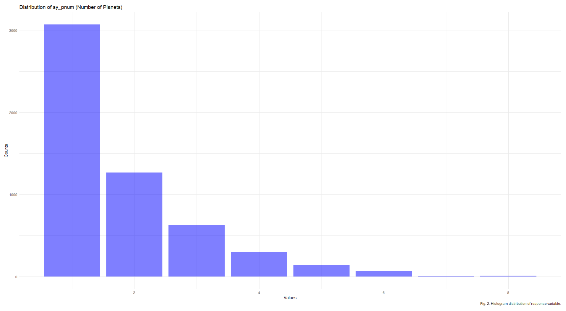
Next, I wanted to check the distribution of the response variable itself: the count of planets in a system. This distribution has a visible right skew, which is expected of this data.

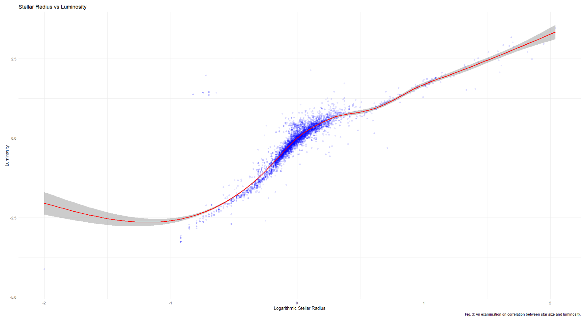
So far so good. Next, it’s useful when looking at data to check and make sure that it follows real-world constraints. When analyzing data on space and exoplanet, these real-world constraints are better known as “physics.” To start with, a larger star is expected to be more luminous, which is confirmed by our data:

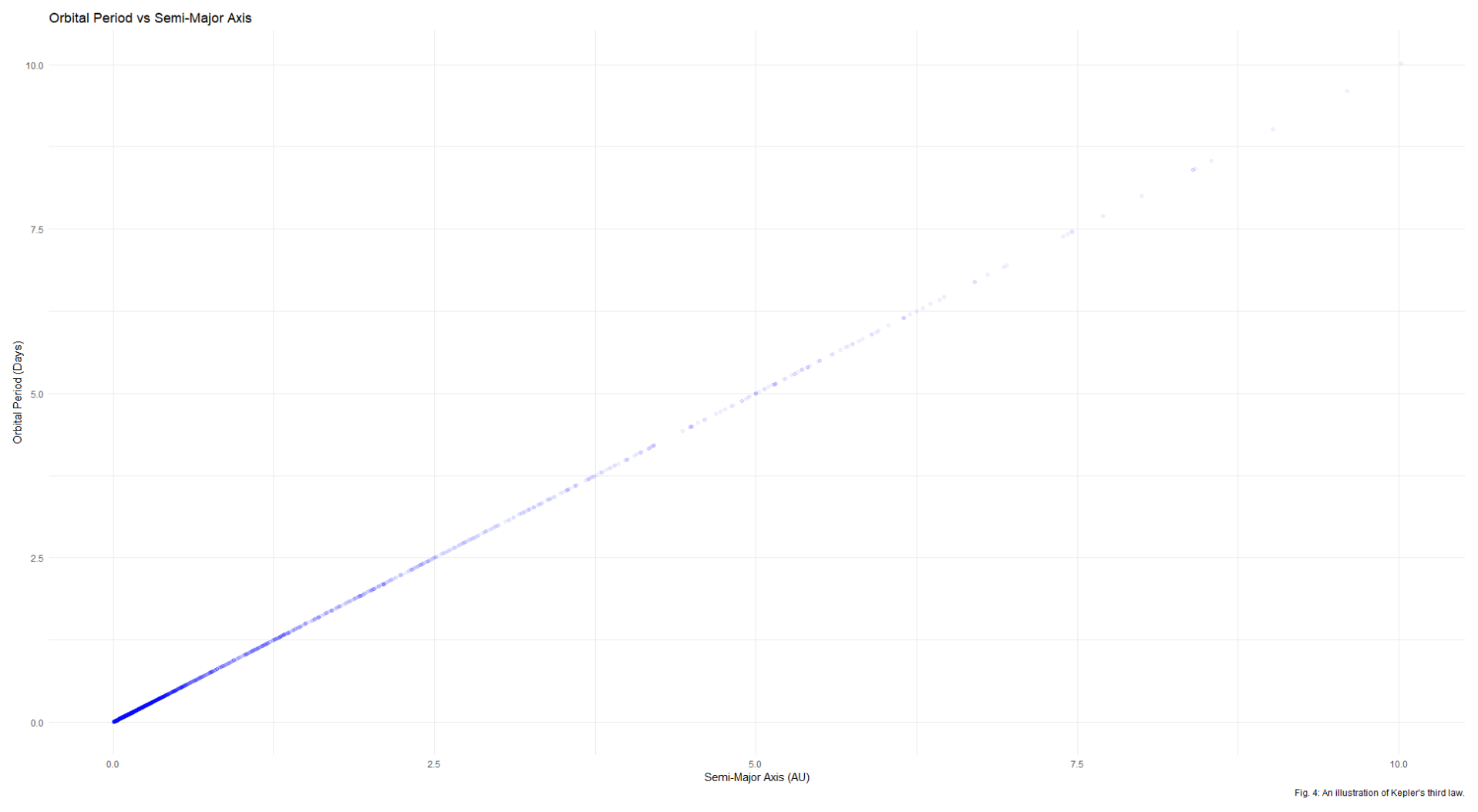
Lastly, Kepler’s Third Law states that the farther a planet is from its star, the longer it takes to orbit that star. There’s an equation for this, making a planet’s orbital period directly proportional to its distance from its host star. This means that a graph comparing the two should be a straight diagonal line:

All of the data looks good and clean in this project - probably because it was directly from NASA - but it’s always good to check.

Statistical Models

There are plenty of different ‘models’ that can be fit to data, depending on the kind of data that someone is working with. The number of exoplanets in a given star system is considered count data (1, 2, 3, etc.), which is largely self-explanatory. Poisson Regression and Negative Binomial Regression are both used for count data.

Poisson Regression is what all count data regression is built on. However, it isn’t often actually applicable, because it assumes that the variance and mean of a given response variable are equal, which just doesn’t happen often. For this data, variance (1.36) and mean (1.80) are actually fairly close.

Negative Binomial models add a dispersion parameter, which is an extra variable that makes them more flexible than Poisson models.

Results (part 1)

Both models actually give nearly identical results. Both include the same significant variables with nearly the exact same significance values. According to our models, stellar metallicity, orbital period, semi-major axis, orbital eccentricity, insolation flux, and stellar density are the most important values that determine the number of exoplanets in a star system.

Variable	Poisson Estimate	Poisson p-value	Negative Binomial Estimate	Negative Binomial p-value
st_met	-0.4569	0.000472 ***	-0.4569	0.000473 ***
pl_orbper	-0.001757	3.89e-07 ***	-0.001757	3.91e-07 ***
pl_orbsmax	1.4170	1.59e-09 ***	1.4170	1.60e-09 ***
pl_orbeccen	-0.6658	0.000377 ***	-0.6658	0.000378 ***
pl_insol	-5.366e-05	0.035062 *	-5.365e-05	0.035101 *
st_dens	0.01413	1.88e-05 ***	0.01413	1.88e-05 ***

Both models also have the same amount of residual deviance - a measure of goodness of fit applied to statistical models.

Model	Residual Deviance
Poisson	660.77
Negative Binomial	660.63

Imputation

There’s one issue with the dataset that I did not include earlier - there’s a lot of missing data. The dataset is built with composite data, meaning it gathers data from multiple telescopes. Some star systems, however, don’t have data for every possible observation. For example, a planet that is captured in multiple telescopes might have data like its stellar metallicity or orbital period, whereas a planet that is only captured in one might have this data missing.

Missing data (and how to handle it) is one of the great problems that plagues data science in general. There are no perfect answers, and any given solution often needs to be justified. For all of the above modeling, I simply removed any row that had any missing data. This removed 1927 out of 5482 rows, or 35%, which is a huge chunk of data.

The second solution to missing data is imputation, which involves filling in any missing data with other, estimated values. There are multiple methods for doing this. The method I used in this project is called KNN, or K-Nearest Neighbor, imputation.

Before imputation:

Planet	st_mass	st_lum	pl_orbeccen	pl_insol
A	1.02	0.95	0.01	1.02
B	0.88	—	0.13	0.78
C	—	1.10	—	1.15
D	1.15	1.08	0.05	0.92
E	0.95	0.87	0.22	—

Row removal keeps only A and D. KNN imputation instead finds the k most similar observations to each incomplete row and fills in the missing value with their average. With k=10, planet B’s missing luminosity gets estimated from the 10 planets whose other measurements look most like B’s:

After KNN imputation:

Planet	st_mass	st_lum	pl_orbeccen	pl_insol
A	1.02	0.95	0.01	1.02
B	0.88	0.91	0.13	0.78
C	0.95	1.10	0.09	1.15
D	1.15	1.08	0.05	0.92
E	0.95	0.87	0.22	0.97

It isn’t perfect, but no method is. My justification for using KNN Imputation in this project is the fact that this dataset works specifically with data grounded in real physics, meaning k similar star systems are actually likely to be able to fill in missing values for others with some level of accuracy.

Results (part 2)

I re-ran Poisson and Negative Binomial models using the new imputed data, and found different results from before. According to the models that use the imputation method, stellar metallicity, orbital eccentricity, and insolation flux are still significant. However, the new models replace orbital period, semi-major axis, and stellar density with star count and stellar luminosity.

Variable	Poisson Estimate (Imputed)	Poisson p-value	Negative Binomial Estimate (Imputed)	Negative Binomial p-value
sy_snum	0.1403	8.07e-07 ***	0.1403	8.09e-07 ***
st_met	-0.1238	0.0324 *	-0.1238	0.0324 *
st_lum	-0.0562	0.0542 .	-0.0562	0.0542 .
pl_orbeccen	-0.3588	2.49e-05 ***	-0.3588	2.49e-05 ***
pl_insol	-1.052e-04	6.35e-10 ***	-1.052e-04	6.37e-10 ***

Again, both models have approximately the same amount of residual deviance.

Model	Residual Deviance
Poisson	3235.1
Negative Binomial	3234.6

I just got two different sets of results from the same dataset, entirely based on how I handled missing data. But which method is better?

Model Comparison

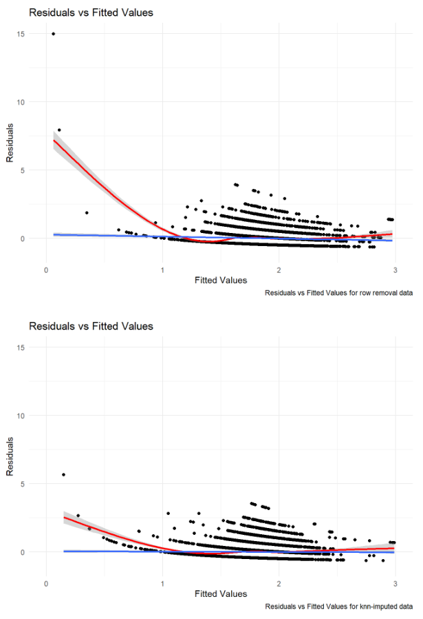
Given that the two types of missing data handling show so much similarity between the models, I decided to compare the simpler Poisson models to one another. This leaves me with two models: A Poisson model where missing data was handled by removing entire rows, and a Poisson model where missing data was handled via imputation.

These models can’t be compared through residual devianace, since there’s a different number of observations in each model. The next best approach is to compare the residuals vs fitted plots. These graphs plot predicted (fitted) values on the x-axis and residuals (errors) in the y-axis. There are several assumptions to be checked and comparisons to be made based on these graphs, and while they are very similar to one another, the model with the imputed data appears just slightly better than the model with removed rows.

Results (part 3)

Using the coefficients given by the Poisson model with imputed data, it’s possible to estimate some real-world ramifications of the data. The coefficients of the five variables shown to be significant are as follows:

Variable	Coefficient Estimate	p-value
sy_snum	0.1447	3.17e-07 ***
st_lum	-0.07634	1.11e-07 ***
st_met	-0.1258	0.023 *
pl_orbeccen	-0.3270	2.44e-05 ***
pl_insol	-1.150e-04	1.04e-12 ***

The coefficients can be interpreted by exponentiating them, giving the following normal language interpretations:

• For each additional star in a system (sy_snum), the expected number of planets increases by 15.57%.
• For each unit increase in stellar luminosity, the expected number of planets decreases by 7.35%.
• For each unit increase in stellar metallicity, the expected number of planets decreases by 11.82%.
• For each unit increase in planetary orbital eccentricity, the expected number of planets decreases by 27.89%
• For each unit increase in insolation flux, the expected number of planets decreases by .01%.

Conclusion

According to the final model, it seems that ‘sy_snum’ (number of stars), ‘st_lum’ (luminosity of stars), ‘st_met’ (stellar metallacity), ‘pl_orbeccen’ (eccentricity of orbit), and ‘pl_insol’ (insolation flux) are the most important factors when determining the number of exoplanets in an star system. These are very intriguing results for the science - some of these factors, like eccentricity, stellar metallicity, and insolation flux are not intuitively tied to the number of planets in a system. Though I’m sure the professionals already know all of this.

Missing data is the greatest area for improvement in my models. The p-significant variables changed depending on how the missing data was accounted for, which could make a big difference when physicists are building real star system computer models.