Can an NBA player’s position be predicted solely from their stats? If so, how accurately?

Background

The NBA is the world’s premier basketball league, and as such, it’s always on the forefront of evolution in the sport. Coaches and analysts often say that the game of basketball is becoming - or has become - ‘positionless’, but is that really true? Is a player’s position really as ambiguous as these experts suggest?

The Data

The dataset for this project is comprised of NBA player statistics for the 2023-2024 NBA basketball season, sourced from Basketball Reference

Lots of cleaning was required to make the dataset usable, since it was web scraped:

1. Tables with multidimensional data were reduced.
2. Columns not including the player name or target variable were converted into numeric.
3. Duplicate entries for players who switched teams midseason were averaged.
4. Tables were joined.
5. Unneeded columns (rank, team, awards, etc.) were removed.
6. Any column names that included characters that the RF model complained about were modified.
7. A new boolean ‘Starter’ column was created, based on whether or not a player started more games than they came off the bench. This is the same metric that the NBA uses to decide who is eligible for the “Sixth Man of the Year” award, which goes to the best non-starter in the league.

If you’re really interested in how that works for some reason, the code is below.

extract_and_process_player_data <- function(year = 2025) {
  library(rvest)
  library(dplyr)
  library(stringr)

  # URLs for Basketball Reference data
  base_url <- "https://www.basketball-reference.com/leagues/"
  urls <- list(
    per_game = paste0(base_url, "NBA_", year, "_per_game.html"),
    per_poss = paste0(base_url, "NBA_", year, "_per_poss.html"),
    advanced = paste0(base_url, "NBA_", year, "_advanced.html"),
    play_by_play = paste0(base_url, "NBA_", year, "_play-by-play.html"),
    shooting = paste0(base_url, "NBA_", year, "_shooting.html"),
    adj_shooting = paste0(base_url, "NBA_", year, "_adj_shooting.html")
  )

  # Reads tables from URL links
  pergame_table <- read_html(urls$per_game) |> html_element("table") |> html_table()
  per100_table <- read_html(urls$per_poss) |> html_element("table") |> html_table()
  advanced_table <- read_html(urls$advanced) |> html_element("table") |> html_table()
  playbyplay_table <- read_html(urls$play_by_play) |> html_element("table") |> html_table()
  shooting_table <- read_html(urls$shooting) |> html_element("table") |> html_table()
  adjustedshooting_table <- read_html(urls$adj_shooting) |> html_element("table") |> html_table()

  # Fixes tables with multidimensional data
  tidy_dimensions <- function(table) {
    table[1, ] <- as.list(paste0(colnames(table), "_", table[1, ]))
    colnames(table) <- table[1, ]
    table <- table[-1, ]
    table <- table %>% rename(Player = `_Player`)
    colnames(table) <- str_remove(colnames(table), "^_")
    return(table)
  }

  playbyplay_table <- tidy_dimensions(playbyplay_table)
  shooting_table <- tidy_dimensions(shooting_table)
  adjustedshooting_table <- tidy_dimensions(adjustedshooting_table)

  # Function to convert every column except 'Player' and 'Pos' into numeric
  convert_except_player_pos <- function(df) {
    df %>%
      mutate(across(
        !any_of(c("Player", "Pos")),
        ~ as.numeric(str_replace_all(., "[^0-9.-]", ""))
      ))
  }

  # Function to average data for each player across their teams
  # On basketball-reference.com, players who play on multiple teams in the same
  # season will sometimes be represented by multiple rows, depending on the table.
  average_aggregate_data <- function(df) {
    df %>%
      group_by(Player) %>%
      summarize(
        Pos = first(Pos),
        across(where(is.numeric), mean, na.rm = TRUE),
        .groups = "drop"
      )
  }

  pergame_table <- convert_except_player_pos(pergame_table)
  advanced_table <- convert_except_player_pos(advanced_table)
  playbyplay_table <- convert_except_player_pos(playbyplay_table)
  shooting_table <- convert_except_player_pos(shooting_table)
  adjustedshooting_table <- convert_except_player_pos(adjustedshooting_table)

  pergame_table <- average_aggregate_data(pergame_table)
  advanced_table <- average_aggregate_data(advanced_table)
  playbyplay_table <- average_aggregate_data(playbyplay_table)
  shooting_table <- average_aggregate_data(shooting_table)
  adjustedshooting_table <- average_aggregate_data(adjustedshooting_table)

  # Joins tables
  players <- pergame_table %>%
    left_join(advanced_table, by = "Player") %>%
    left_join(playbyplay_table, by = "Player") %>%
    left_join(shooting_table, by = "Player") %>%
    left_join(adjustedshooting_table, by = "Player") %>%
    select(-ends_with(".y")) %>%
    select(-ends_with(".x.x")) %>%
    select(-ends_with(".x.y"))

  # Gets rid of duplicate and/or irrelevant columns
  players <- players %>%
    select(-starts_with("Rk"),
           -starts_with("Age"),
           -starts_with("Team"),
           -starts_with("Awards"),
           -MP,
           -starts_with("Position"))

  colnames(players) <- str_remove(colnames(players), "\.x$")
  players <- players[, !duplicated(names(players))]

  # Removes any characters that the RF model errors on
  colnames(players) <- colnames(players) %>%
    str_replace("^\\+/-", "PlusMinus_") %>%
    str_replace("^2", "Two_") %>%
    str_replace("^3", "Three_") %>%
    str_replace("%$", "_pct") %>%
    str_replace_all("%", "pct") %>%
    str_replace_all("[/]", "_") %>%
    str_replace_all("\\.", "_") %>%
    str_replace_all("-", "_") %>%
    str_replace_all("\\+", "_plus")

  players <- players %>% filter(Player != "League Average")
  players <- players %>% rename_with(~ str_replace_all(.x, " ", "_"))

  # Creates new variable "Starter"
  players <- players %>%
    mutate(Starter = ifelse(is.na(G), "NA",
                            ifelse(is.na(GS), "NA",
                                   ifelse(G - GS < GS, "Starter", "Non-Starter"))))

  return(players)
}

Exploratory Data Analysis (EDA)

In basketball, the point guard’s role is usually to initiate the offense, start plays, and pass well. We see this in the distribution of assists per 100 possessions:

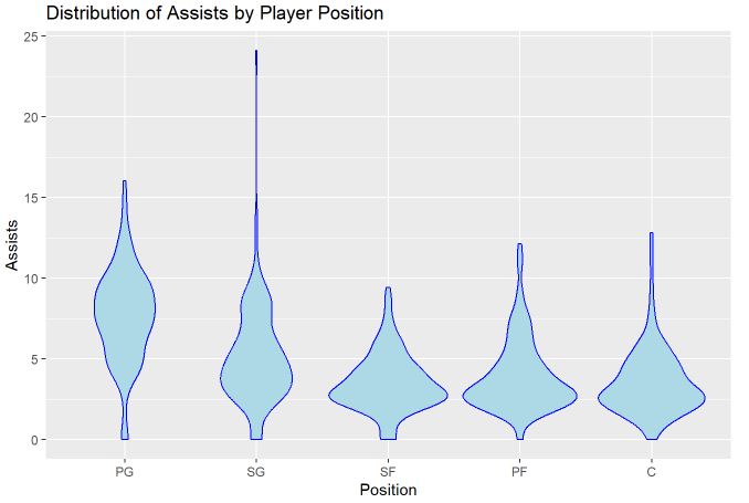
One thing to note: That singular shooting guard averaging 24 assists per 100 possessions is Marquis Nowell, who checked into 1 game for 4 minutes and had 2 assists. The dataset includes some more outliers like that, including Adam Flagler (14 total minutes played, 13.7 assists per 100 possessions) and JD Davison (39 minutes played, 12.7 assists per 100 possessions). Handling players with low minutes is discussed in #reflection

(Also, when I submitted this assignment for class, I said that chart was per-game rather than per 100 possessions, which doesn’t make a lot of sense given how many point guards in the distribution were averaging over 10 assists. My professor didn’t notice. Sorry Dr. Kleffner, if you see this.)

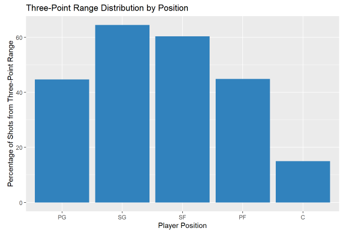
This bar schart shows the percentage of field goal attempts taken from beyond the three point-line as opposed to within the arc. It makes sense that the shooting guard position would take the highest percentage of their shots from behind the line, but it’s interesting to see that the three makes up about the same percentage of a point guard’s shot diet as a power forward. That is probably something that’s changed from 20 years ago.

Modeling

The model used in this project is called a random forest. A random forest is made up of decision trees, which are pretty simple to understand. A decision tree is a sort of flowchart that makes a classification decision by asking a series of yes/no questions. A decision tree for basketball statistics might look like:

Is assists per 100 possessions > 7?
├── Yes → Is three-point attempt rate > 45%?
│         ├── Yes → Shooting Guard
│         └── No  → Point Guard
└── No  → Is blocks per 100 possessions > 2?
          ├── Yes → Center
          └── No  → Power Forward / Small Forward

Decision trees are intuitive, but they have a well-known flaw: they tend to overfit. A single tree memorizes the training data too well and struggles to generalize. It loses nuance - Josh Hart is a small forward who grabs a ton of rebounds, but if a decision tree set a strict cutoff like “if a player averages 8 rebounds, they’re a center or power forward” it would miss Hart.

A Random Forest fixes this issue by building hundreds of trees, each one trained on a random sample of the data and allowed to look at only a random subset of the available stats. Each tree votes on what position a player is, and the whatever position wins the majority of votes wins.

The “random” in Random Forest refers to two sources of randomness:

1. Bootstrapping — each tree trains on a random sample (with replacement) of the players in the dataset.
2. Feature sampling — at each split, the tree can only consider a random subset of stats, rather than all of them at once.

This randomness forces the trees to be different from each other, which is what makes the forest powerful.

Evaluation

I was a bit surprised by the model underperforming compared to my expectations. I figured that with so many statistics to go off of, the model would be able to classify players at a very high rate.

However, while the model wasn’t the strongest, it certianly wasn’t weak either. The Confusion Matrix below bears a sharper orange up the diagonal .45 than to the corners, but there’s a good amount of error.

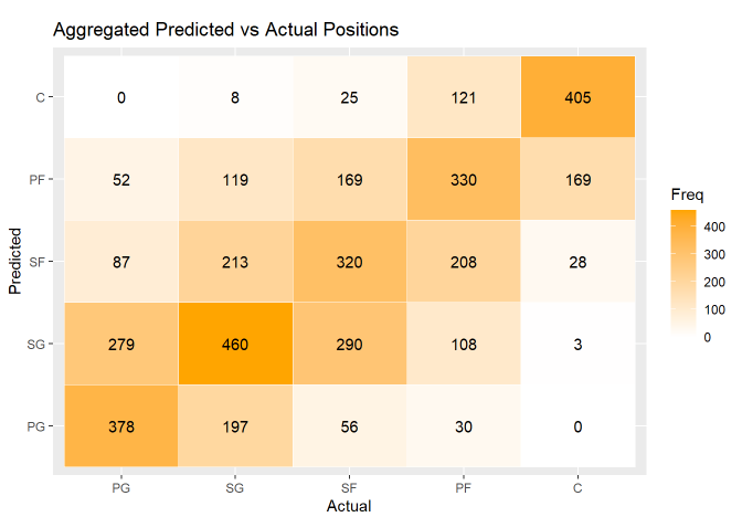
Aside from just accuracy (whether the model got a pick right or wrong), we can also measure how far off the model was on average. Treating basketball positions as ordinal categorical data points, we can use the Quadratic Weighted Kappa (QWK) to measure how far off the model was on average.

• Mean Model Accuracy: 46.69%
• Mean Quadratic Weighted Kappa: 0.7057

We can also look at which variables the model decided was most important to guessing which position a player played. There are some interesting results - rebound-related statistics make up 5/10 of the most important variables, whereas shooting-related statistics only make up 4/10.

The data certainly seems to suggest a somewhat “positionless” game, but there’s an even better way to check.

20-Year Comparison

When the exact same analysis is run on data from 2003-2004, the new model actually performs better - meaning it’s better at predicting which position a player plays based on their stats.

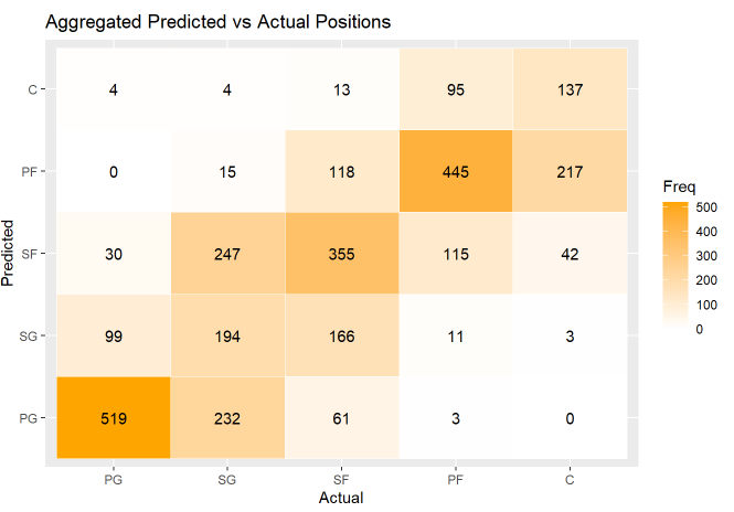
Conclusion & App

This analysis actually lends a lot of credit to the idea that basketball has become more positionless over the years - if it’s more difficult to guess a player’s position now than 20 years ago, it means that more players are being asked to play roles typically filled by other positions.

I could have (probably should have) added a minutes requirement, since some players with few minutes but high per-36 and per-100-possessions stats probably skew the model.

The analysis above is also available as a Shiny app, which you can access at this link to perform the analysis yourself: NBA Player Analysis and Bootstrapping